Linear Static and Vibration Analysis of Bernoulli Frames
This notebook demonstrates how to use pyaxisvm to build and analyze 3d frames. We will build a scalable model, consisting of a grid of Bernoulli beams, and perform a linear static analysis and a linear vibration analysis. We will use NumPy to store and handle numerical data and PolyMesh for grid generation.
Input Data
Python has a waste number of third party packages, that might save you dozens of time. Now we are going to use the PolyMesh library to create a grid of lines. The following lines contain all input parameters of the calculations. After modifying these, the rest should work.
[1]:
# the size of the grid
Lx, Ly, Lz = 10., 2.0, 1.0

# these control subdivision
# set these higher if you want more lines in the same space
nx, ny, nz = 4, 2, 2

# data of a CHS section
D = 0.1  # outer diameter of the tube in m
t = 0.05  # thickness of the tube in m

# value of the concentrated force at the free end in kN
# and the number of load cases to generate
F = 1.0
nCase = 5
Mesh Creation
We can create a 3d grid of bernoulli beams using the PolyMesh library. After it, we are going to have our mesh as two NumPy arrays, coords for the coordinates and topo for nodal connectivity. We will use these to build our AxisVM model.
[2]:
from polymesh.space import StandardFrame, PointCloud
from polymesh.grid import gridH8 as grid
from polymesh.utils.topology.tr import H8_to_L2
import numpy as np

# mesh
gridparams = {
    'size': (Lx, Ly, Lz),
    'shape': (nx, ny, nz),
    'origo': (0, 0, 0),
    'start': 0
}

# create a grid of hexagonals
coords, topo = grid(**gridparams)

# turn the hexagonal mesh into lines
coords, topo = H8_to_L2(coords, topo)

GlobalFrame = StandardFrame(dim=3)

# define a pointcloud
points = PointCloud(coords, frame=GlobalFrame).centralize()

# set the origo to the center of the fixed end
dx = - np.array([points[:, 0].min(), 0., 0.])
points.move(dx)

# get the coordinates of the vectors
coords = points.show()
AxisVM
Starting an AxisVM instance is easy. If in a Jupyter Notebook, drop the interface and watch a html represantation of it, which summarizes the version of the application and the type library as well.
[3]:
from axisvm.com.client import start_AxisVM
axvm = start_AxisVM(visible=True, daemon=True)
axvm
[3]:
| IAxisVMApplication | Information |
|---|---|
| AxisVM Platform | 64 bit |
| AxisVM Version | 15 r4r En 0 |
| Type Library Version | 15 401 |
[4]:
import axisvm.com.tlb as axtlb

# create new model
modelId = axvm.Models.New()
axm = axvm.Models[modelId]

# material
ndc, material = axtlb.ndcEuroCode, "S 235"
axm.Settings.NationalDesignCode = ndc

# cross section
MaterialIndex = axm.Materials.AddFromCatalog(ndc, material)
CrossSectionIndex = axm.CrossSections.AddCircleHollow('S1', D, t)

# crate nodes
fnc = axm.Nodes.Add
list(map(lambda c: fnc(*c), coords))

# create lines
fnc = axm.Lines.Add
GeomType = axtlb.lgtStraightLine
list(map(lambda x: fnc(x[0], x[1], GeomType), topo + 1))

# set material and cross section
LineAttr = axtlb.RLineAttr(
    LineType=axtlb.ltBeam,
    MaterialIndex=MaterialIndex,
    StartCrossSectionIndex=CrossSectionIndex,
    EndCrossSectionIndex=CrossSectionIndex
)
lineIDs = [i+1 for i in range(axm.Lines.Count)]
attributes = [LineAttr for _ in range(axm.Lines.Count)]
axm.Lines.BulkSetAttr(lineIDs, attributes)

# nodal supports
spring = axtlb.RStiffnesses(x=1e12, y=1e12, z=1e12, xx=1e12, yy=1e12, zz=1e12)
RNonLinearity = axtlb.RNonLinearity(
    x=axtlb.lnlTensionAndCompression,
    y=axtlb.lnlTensionAndCompression,
    z=axtlb.lnlTensionAndCompression,
    xx=axtlb.lnlTensionAndCompression,
    yy=axtlb.lnlTensionAndCompression,
    zz=axtlb.lnlTensionAndCompression
)
RResistances = axtlb.RResistances(x=0, y=0, z=0, xx=0, yy=0, zz=0)
ebcinds = np.where(coords[:, 0] < 1e-12)[0]
for i in ebcinds:
    axm.NodalSupports.AddNodalGlobal(spring, RNonLinearity, RResistances, i+1)

# nodal loads
load_cases = {}
LoadCaseType = axtlb.lctStandard
inds = np.where(coords[:, 0] > Lx - 1e-12)[0] + 1
axm.BeginUpdate()
for case in range(nCase):
    name = 'LC{}'.format(case+1)
    lcid = axm.LoadCases.Add(name, LoadCaseType)
    pid = np.random.choice(inds)
    Fx, Fy, Fz = 0, 0, -F
    force = axtlb.RLoadNodalForce(
        LoadCaseId=lcid,
        NodeId=pid,
        Fx=Fx, Fy=Fy, Fz=Fz,
        Mx=0., My=0., Mz=0.,
        ReferenceId=0
    )
    axm.Loads.AddNodalForce(force)
    load_cases[lcid] = dict(name=name, id=case)
axm.EndUpdate()

# save the model before calculation
fpath = 'the_name_of_your_file.axs'
axm.SaveToFile(fpath, False)
axm
[4]:
| IAxisVMModel | Information |
|---|---|
| N Nodes | 45 |
| N Lines | 96 |
| N Members | 96 |
| N Surfaces | 0 |
| N Domains | 0 |
Linear Static Analysis
We can perform a linear elastic static analysis with the following command:
[5]:
axm.Calculation.LinearAnalysis(axtlb.cuiNoUserInteractionWithAutoCorrectNoShow)
[5]:
1
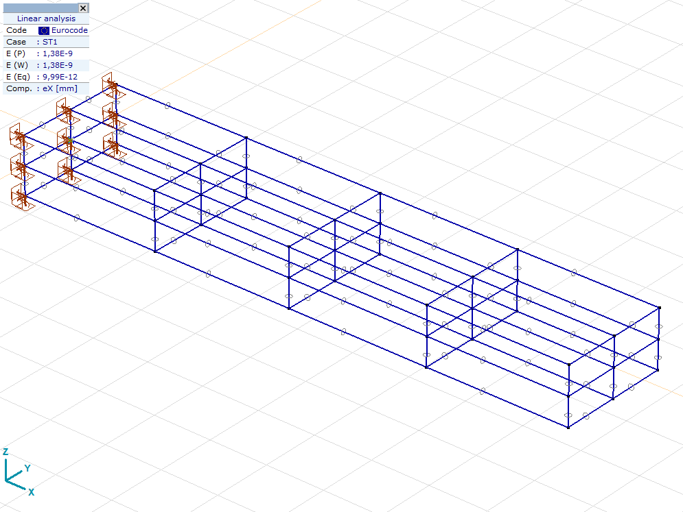
You can make a screenshot anytime!
[6]:
axvm.BringToFront()
axm.View = axtlb.vPerspective
axvm.MainFormTab = axtlb.mftStatic
axm.FitInView()
axm.Windows[1].screenshot()
[6]:
The following block fetches displacements for all nodes and load cases in the model and stores it in a NumPy array. You can use this block as a template in any of your future workflows.
[7]:
disps = axm.Results.Displacements
disps.DisplacementSystem = axtlb.dsGlobal
disps.LoadLevelOrModeShapeOrTimeStep = 1
dofsol = np.zeros((axm.Nodes.Count, 3, nCase))
for lcid, lcdata in load_cases.items():
    lcname = lcdata['name']  # retrieve the name of the load case
    disps.LoadCaseId = lcid
    load_case_id = lcdata['id']
    for nodeId in range(axm.Nodes.Count):
        d = disps.NodalDisplacementByLoadCaseId(i+1)[0]
        dofsol[nodeId, 0, load_case_id] = d.ex
        dofsol[nodeId, 1, load_case_id] = d.ey
        dofsol[nodeId, 2, load_case_id] = d.ez
dofsol[np.where(np.abs(dofsol) < 0.00001)] = 0.0  # trim very small values
The array has values for all 45 nodes, 3 spatial dimensions and 5 load cases
[8]:
dofsol.shape
[8]:
(45, 3, 5)
Vibration Analysis
The following block performs a vibration analysis for the first load case.
[9]:
options = axtlb.RVibration(
    LoadCase = 1,
    Iterations = 30,
    ModeShapes = 15,
    EigenValueConvergence = 1e-3,
    EigenVectorConvergence = 1e-3,
    MassControl = axtlb.mcMassesOnly,
    ConvertLoadsToMasses = False,
    ConcentratedMasses = False,
    ConvertConcentratedMassesToLoads = False,
    ElementMasses = True,
    MassComponentX = True,
    MassComponentY = True,
    MassComponentZ = True,
    ConvertSlabsToDiaphragms = False,
    MassMatrixType = axtlb.mtConsistent,
    IncreasedSupportStiffness = False,
    MassesTakenIntoAccount=axtlb.mtiaAll
)
interaction = axtlb.cuiNoUserInteractionWithAutoCorrectNoShow
axm.Calculation.Vibration(options, interaction)
[9]:
[<comtypes.gen._0AA46C32_04EF_46E3_B0E4_D2DA28D0AB08_0_16_100.RVibration at 0x209214212c0>,
 1]
Execute this line to get the natural circular frequencies:
[10]:
freks, _ = axm.Results.GetAllFrequencies(axtlb.atLinearVibration, 1)
freks
[10]:
(2.959385451831059,
 3.0874871771922074,
 4.2843169427821906,
 9.185151639376052,
 9.515214328710275,
 12.974291945228083,
 15.96847008498523,
 16.552764989633506,
 21.82392993055216,
 21.869449619700013,
 22.11765361461048,
 28.831941430030103,
 61.843802681433814,
 63.1993862629429,
 67.8132972985758)
You can also get modal mass factors. It is easy to read out from the results, that the first two modes correspond to bending shapes.
[11]:
records, _ = axm.Results.GetAllModalMassfactors(axtlb.atLinearVibration, 1)
records = np.array([[r.x, r.y, r.z] for r in records])
records[np.where(records < 0.001)] = 0.0  # rule out small values
records *= 100  # to get percentage values
records
[11]:
array([[ 0.        , 74.60765839,  0.        ],
       [ 0.        ,  0.        , 74.40606356],
       [ 0.        ,  0.        ,  0.        ],
       [ 0.        ,  8.9579545 ,  0.        ],
       [ 0.        ,  0.        ,  9.68592092],
       [ 0.        ,  0.        ,  0.        ],
       [ 0.        ,  2.84366924,  0.        ],
       [ 0.        ,  0.        ,  2.56371368],
       [ 0.        ,  0.        ,  0.        ],
       [ 0.        ,  0.7027301 ,  0.        ],
       [ 0.        ,  0.        ,  0.55825803],
       [ 0.        ,  0.        ,  0.        ],
       [ 0.        ,  0.        ,  0.        ],
       [ 0.        ,  0.        ,  0.        ],
       [ 0.        ,  0.        ,  0.        ]])
Finally, close AxisVM if you are done.
[16]:
axvm.Quit()